
Table of contents
- What a bond is and how its yield is composed
- The concept of the term structure of interest rates and its determinants
- The three types of yield curves
- Theories explaining the shape of the term structure of interest rates
- The current extreme situation with respect to the inversion of the yield curves
- How to bet on steepening yield curves
- Conclusion
What a bond is and how its yield is composed
Various entities like states or corporations can issue bonds in the capital markets to fund themselves. Thereby, the investor pays the issuer a price for the bond and in return receives a certain predetermined notional amount back when the bond reaches its maturity. Additionally, the issuer may regularly disburse a coupon to the investor if applicable.
The issuer’s creditworthiness at the time of the bond’s placement, the then prevailing economic circumstances and the resultant demand for as well as supply of bonds from comparable issuers, in conjunction with future prospects determine, inclusive of further factors, the yield of a bond. This rate of return serves as a measure to quantify how high the investor’s annual relative return is.
The influence of these factors is reflected by several components which basically make up the bond’s yield. The basis is the so-called “risk-free” interest rate, namely the yield of a bond with a very short time to maturity of an issuer whose creditworthiness is considered so high that the risk of default on a payment is practically neglected, although this possibility cannot be completely ruled out. Depending on the investor’s focus and the bond’s currency, various issuers can be considered for this role. In principle, countries such as the USA and Germany are used.
Any other components are assessed as premia on this “risk-free” interest rate. For instance, this also includes the credit risk. The higher the risk that the issuer will not meet its payment obligations in the future, the higher is the premium for this. Furthermore, if the liquidity of the bond is low because either the supply or the demand for it is too low, investors demand a compensation for the limited tradability. Moreover, if market participants expect the inflation rate to be higher in the future, they also demand a yield premium for this aspect.
The issuer decides how long the term of the bond should be based on his financial needs and the expected relative costs. This time to maturity determines when the bond’s notional amount is repaid to the investor. This period ranges from a few days in extreme cases, to a few years in normal cases, to several decades. Some special bonds whose notional value is not redeemed and for which the investor only receives coupon payments have no maturity date at all and are therefore also referred to as perpetual bonds.
The last of the most significant risk components in this context is the yield premium for the duration of the capital commitment. The longer the bond’s time to maturity is, the higher is also usually the compensation. This is due to the fact that a bond with a long maturity is normally also more sensitive to changes in the market interest rate. To the risk components listed above, one could add others, depending on the regarded theory of the term structure of interest rates.
The concept of the term structure of interest rates and its determinants
A term structure of interest rates (hereafter referred to as the yield curve) depicts the annualised yield as a percentage depending on the remaining time to maturity of the bonds of the same issuer, usually represented in years. The most common variant of the yield curve is the one with spot interest rates, i.e., the yield that would be received if the bond were to be purchased at the current price.
The yield curve’s shape and changes to it due to macroeconomic events (e.g., an increase or decrease in the key interest rate decided by the central bank) are generally covered by three characteristics of the yield curve: the level, the slope and the curvature.[1]
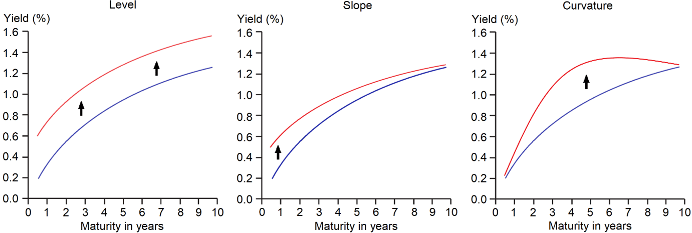
Figure 1: The three characteristics of the term structure of interest rates. The yield curves are symbolic and the yields are annualised. Changes in the level of yields of certain tenor areas are represented with arrows.
The level of a yield curve, when viewed in isolation, initially has a limited information content, namely merely at which level the yields of the respective issuer are. Only with the addition of another yield curve can further insights be derived. If one compares the yield curve of an issuer with that of the same one but from a different day, one can recognize the change in level over time. If one compares it with that of another issuer, the following rule emerges: the higher (lower) the yield curve of one issuer is relative to that of another, the more positive (negative) the risk premium is, ceteris paribus.
The left-hand diagram in Figure 1 illustrates an increase in the level of the yield curve. This is the case where the curve shifts vertically upwards parallel to its initial position (blue) to re-manifest itself at a higher level (red). Ideally, the absolute change in the yield level is the same for all tenors. Similarly, the yield curve could also shift parallel downwards so that a lower level is reached.
The steeper an ascending (descending) yield curve is, the higher (lower) is, ceteris paribus, the incremental yield premium for the duration of the capital commitment of a tenor relative to the previous tenor. Thus, the slope of a yield curve essentially reflects the incremental return premium between the yield curve’s tenors. This implies that a yield curve, which is perfectly horizontal, exhibits no additional yield premium between tenors, ceteris paribus.
The middle diagram in Figure 1 depicts one of the four variants of a change in the slope respectively steepness of the yield curve, in this case a flattening. To be precise, this is a so-called “bear flattener”. The name derives from the fact that this type of change in the yield curve precedes an increase in the key interest rate on the part of the central bank, which thereby aims to counteract an increase in the inflation rate. This measure has a negative effect on both the respective local economy as well as stock market and is therefore called a “bearish flattening”. In this case, the yields of short-term maturities, which the key interest rate influences the most, rise more strongly than those of long-term maturities.
Thus, whilst yields on short-term maturities are directly influenced by the central bank through the policy rate, yields on long-term maturities are not directly controllable by such a discrete instrument of monetary policy. Instead, the yields of longer tenors are determined by expectations about the development of future short-term yields, inflation, economic activity and the path of the policy rate.
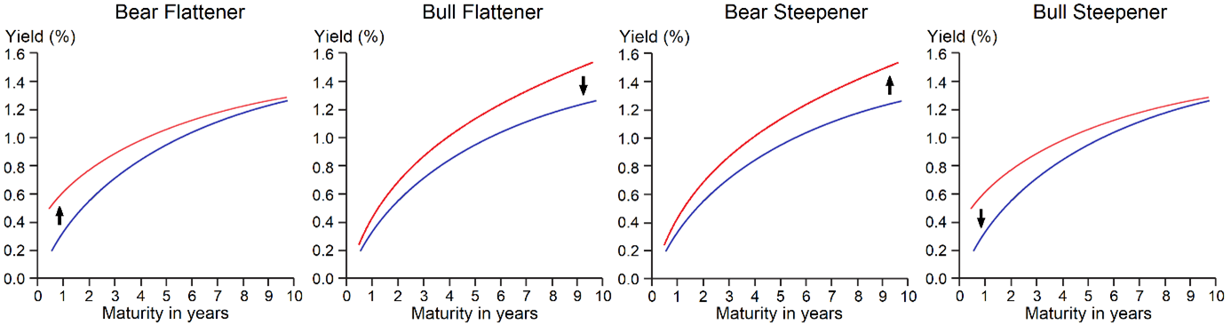
Figure 2: The four variants of a change in the slope of the yield curve. The yield curves are symbolic and the yields are annualised. Changes in the level of yields of certain tenor areas are represented with arrows.
The second variant, namely the counterpart to the one described above, is the “bull-flattener”, i.e., the second possibility of a flattening of the yield curve (second diagram in Figure 2). In this case, the yields of long-term maturities fall faster than those of short-term maturities. This might happen if investors are looking for a safe haven in uncertain times or if the expected level of future inflation falls. In such scenarios, the central bank lowers the key interest rate to support the economy. Since such a move is also beneficial for the stock market, it is called a “bullish flattening”.
The opposite of the flattening of the yield curve is its steepening, which covers the third and fourth variants of a change in the slope of the yield curve. In the case of a bear steepener (third diagram in Figure 2), long-term yields rise more than short-term yields as the expected level of future inflation rises and market participants begin to anticipate an increase in the policy rate. With a bull steepener (fourth diagram in Figure 2), yields on short-term maturities fall faster than those on long-term maturities as the expectation of a reduction in the policy rate increases.
Compared to the yield curve’s slope, which only covers the relationship between the yields of short-term and long-term maturities, its curvature (right-hand diagram of Figure 1) also incorporates the yields of medium-term maturities in this consideration. In the case that the yield curve forms a perfect straight line (note the contradiction in nomenclature), there is no curvature. In this regard, the slope is irrelevant. This implies that a distinction is made between two types of curvature: A positive (negative) curvature exists if the yields of the medium-term maturities lie above (below) the hypothetical straight line formed by the short- and long-term yields.
There are multiple macroeconomic interpretations of the yield curve’s curvature. One view is that it reflects the cyclical fluctuations of the economy and that the decline of a positive curvature towards a straighter yield curve seems to anticipate or accompany a weakening of the economy. Empirically, a period of strong positive curvature is accompanied by a period of low unemployment.[2]
A similar empirical implication is that an unexpected strengthening of the positive curvature is followed by a sharp increase in the yields of short-term maturities, while those of long-term maturities remain unchanged. This causes the yield curve to flatten over time, which is associated with a reduction in economic output.[3]
The three types of yield curves
Depending on the current as well as expected macroeconomic conditions and on the consequent expression of the three characteristics of the yield curve, three different types of the yield curve can establish themselves, which are discussed in more detail below. These can be observed in the course of economic cycles, whereby it may well take several years for the curve to transform from one type to the next. Figure 3 illustrates the three types.
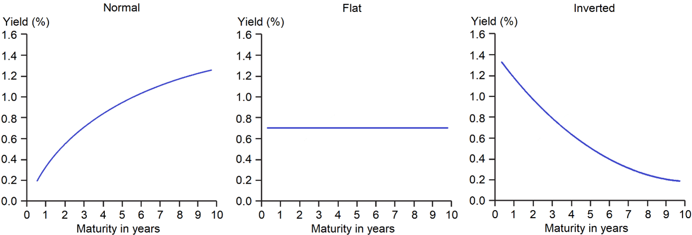
Figure 3: The three types of yield curves. The yield curves are symbolic and the yields are annualised. Source: Own chart.
The most commonly observed type is called the normal yield curve and is shown in the left-hand diagram of Figure 3. An issuer can, as already explained, bring bonds with different maturity dates to the market. All of the above stated yield components are positively correlated with the maturity. This implies that, normally, higher yields are demanded with an increasing tenor. Therefore, this type of the yield curve is also called normal. Typically, the normal yield curve is concave and, in the theoretical ideal case, even strictly monotonically increasing (i.e., the yields of the short-term tenors are lower than those of the medium-term, which in turn are lower than those of the long-term). A normal curve is mostly observed during the phase of an economic expansion, thus when economic growth and the inflation rate are rising.
As already explained, a yield curve can flatten due to a bear or bull flattener if the yield curve was normal before. In the theoretical ideal case, the level of return is then the same for all tenors (middle diagram of Figure 3). However, if the effect of the flattening is much stronger than the yield curve just flattening, the curve may even invert. This is the opposite case of a normal yield curve, so that the yield curve is convex and falling (right diagram of Figure 3). In such a situation, the returns of the short-term tenors are thus higher than those of the medium-term, which in turn are higher than those of the long-term.
An inverse yield curve can occur when market participants expect the future policy rate to be lower than the current one, i.e., when the central bank is likely to lower it soon. Historically, the yield curve has often been inverted in some countries, most prominently the USA, before an economic contraction has occurred.
Based on an inverse yield curve, a steepening of the yield curve can also set in again, this time with the effects of the previously described bear or bull steepener appearing. Thus, the case of a flat yield curve represents a transition phase between a normal and an inverse yield curve.
Theories explaining the shape of the term structure of interest rates
There are several theories which attempt to explain the actual expression of the yield curve. One of them, which also constitutes the basis for some of the others, is the “theory of pure expectations”. In essence, it states that the shape of the yield curve is determined solely by the expectations of market participants and that the yields of long-term maturities correspond to the mean value of future, expected yields of short-term maturities. Thus, this theory is based on the assumption of risk neutrality, i.e., that market participants do not demand a risk premium if the maturity of the bond is not consistent with their investment horizon. If the curve is normal (inverse/flat), this theory predicts that the yields of short-term maturities will be higher (lower/equal).
A variation is the “theory of local expectations”. In contrast to the previous theory, this one states that risk neutrality only applies to short-term maturities. This implies that there should exist a positive risk premium for long-term maturities. However, empirically, it can be shown that this theory does not hold due to liquidity risk premia.
The “liquidity preference theory” complements the “theory of pure expectations” by assuming that forward interest rates correspond to the expected future spot interest rates plus a liquidity risk premium which increases with the time to maturity. In this context, the forward rate represents an interest rate that is determined today but will eventually be applied in the future. In this case, creditors only prefer to lend in the short term, while debtors favour to borrow on a long-term basis. If the yield curve is inverted, this theory predicts that future yields on short-term maturities will become lower.
Another derivative of the ” theory of pure expectations” is the “preferred habitat theory”. It is similar to the “liquidity preference theory“ but rejects that the liquidity risk premium depends on the maturity. Instead, it proposes that in the event of a demand-supply mismatch on their preferred tenor, issuers and investors will switch to alternative tenors with the opposite mismatch, but will require a compensation for this through the yield. This implies that the tenors can exhibit different risk premia. The advantage of this is that this theory can explain all types of the yield curve.
A completely different theory, which is not based on investors’ expectations, is the “market segmentation theory”. In this case, the balance between the demand and supply for a certain tenor essentially determines how high the associated yield turns out to be. This implies that the return of each tenor establishes itself independent of the other tenors. An assumption of this view is that many market participants trade only on certain tenors because other tenors are not an option for them for a variety of reasons. An example of this are pension funds which primarily focus on long-term bonds.
The current extreme situation with respect to the inversion of the yield curves
As of the end of December 2022, the yield curves of many sovereign issuers are far from being able to be described as normal. The cases of Germany and the USA are examined in more detail below.
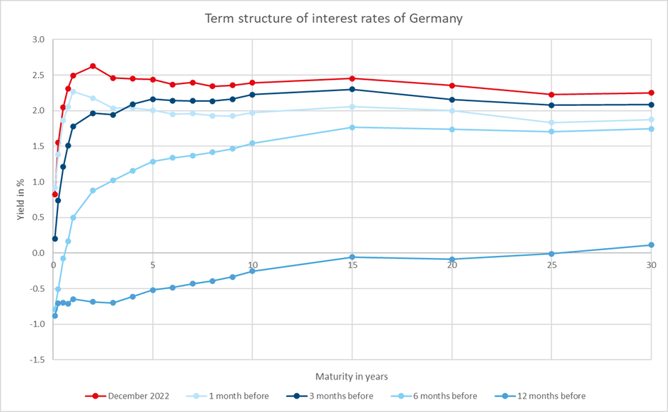
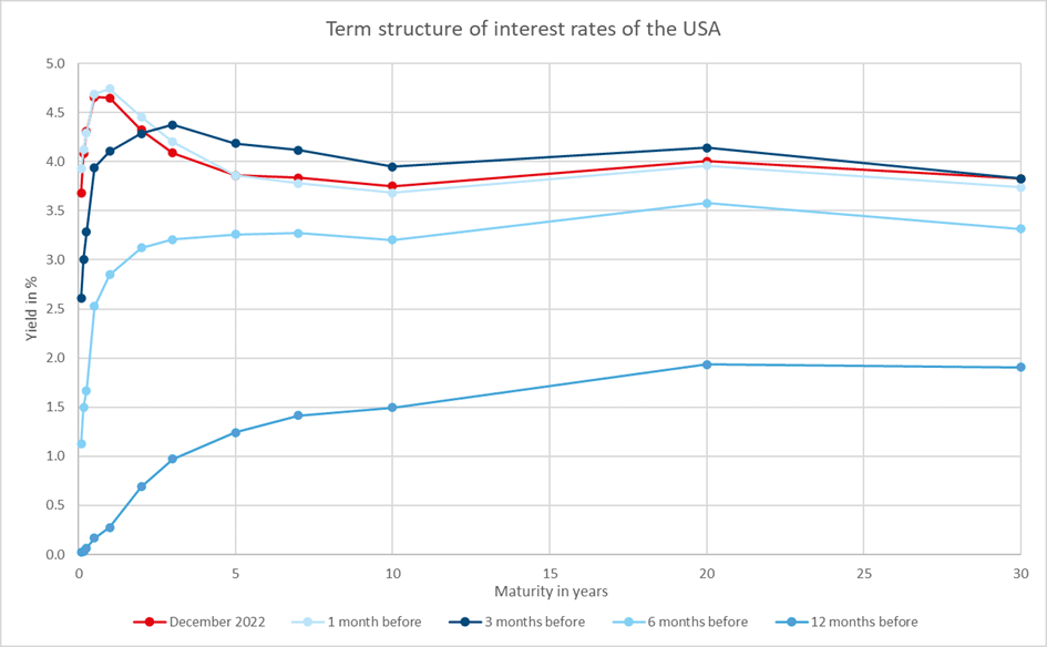
Figure 4: The term structures of interest rates of Germany and the USA (as of December 2022). The returns are annualised. The red graphs represent the curves as of December 2022 and serve as a reference point, whereas the other curves reflect the situations of the past months. Source: Own graph with data from Bloomberg.
The upper diagram in Figure 4 illustrates the development of the German yield curve over time, using December 2022 as a reference point. Six months earlier, the yield curve was still quite normal up until the 15-year tenor, but recently (red graph), it has been very steep in the range of the intra-year tenors, whereas the section of the curve from one year onwards is partly inverted and partly flat. It can be observed that over the preceding twelve months the level has risen continuously and the yield curve has completely moved away from the negative territory, while the curvature has become more and more positive. The situation is similar for the USA (lower diagram of Figure 4). Here, the inversion of the yield curve has recently been even more pronounced. The increase in the level and the strengthening of the curvature over the last year is also clearly visible.
To visualise how extreme the flattening of the yield curves currently is for both issuers, one can examine the spread, i.e., the difference, between the yields of the long-term and short-term maturities. Several combinations are possible. The most common spread is that between the ten-year and two-year tenor, which reflects the steepness of the left half of the yield curve. Similarly, the spread between the 30- and ten-year tenors is representative of the right half. To get an idea of the steepness of almost the entire yield curve, the spread between the 30-year and two-year tenors is considered below.
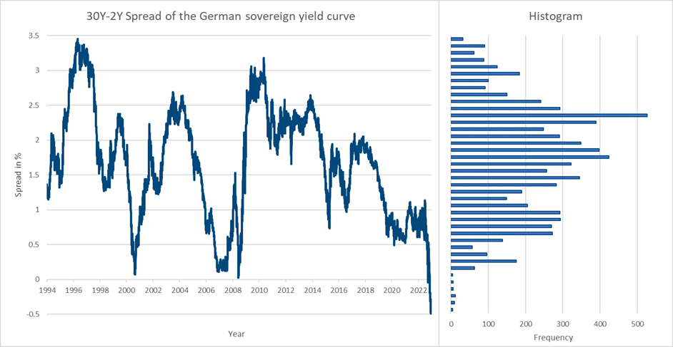
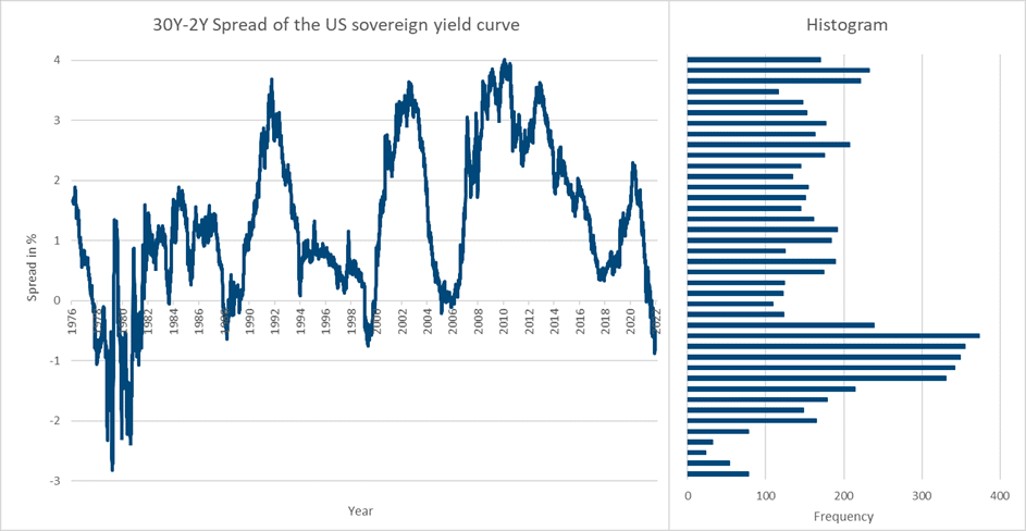
Figure 5: The historical development of the spreads between the yields of the 30-year and two-year tenor of Germany and the USA and their distributions (as of December 2022). The returns are annualised. The graphs and the histograms use the same ordinate, respectively. The bins of the histograms have a width of one tenth of one percent.
The upper diagram in Figure 5 depicts the historical development of the spread between the yields of Germany’s 30-year and two-year tenors, whereas the lower diagram illustrates the one of the USA. It can be noted that in the case of Germany, according to the data available from 1994 onwards, the lowest value (circa -0.5%) has currently been reached for this spread. The latter had almost reached zero in 2000, 2007 and 2008, but became negative for the first time in 2022. It ranges from the current minimum of -0.5% to the historical maximum of approximately +3.5% and thus has a range of 4%.
Considering the corresponding histogram, it becomes clear that the current inversion of the spread represents a so-called “fat-tail” event, i.e., that a scenario has been reached which only appears in extremely exceptional situations. With a mean value of 1.68% and a standard deviation of 0.78% as of December 2022, at that time, the value of the spread has been -2.78 standard deviations away from the mean value. Assuming that the spread in the case of Germany is approximately normally distributed, as can be inferred from the histogram, and considering that three standard deviations in normal distributions cover 99.7% of all observations, the present case also statistically represents an extreme situation.
In the case of the USA (lower chart of Figure 5), the situation is similar but still slightly different. In the late 1970s, the spread almost reached -3%, setting the bar very low for extrema. Thereafter, the spread inverted in 1988, 1999, 2005/2006 and again in 2022, with the spread remaining above a value of -1% in these cases. The spread ranges from the historical minimum of -3% to the historical maximum of approx. +4% and thus has a range of 7%.
Depending on how quickly the Federal Open Market Committee of the Federal Reserve System, i.e., the central banking system of the USA, manages to bring down the currently very high inflation rate via the adjustment of the key interest rate including further monetary policy measures, the inversion of the spread could increase further and at least approach the levels of the late 1970s. Since the distribution of the observations of the spread for the USA is rather evenly distributed, an interpretation via the standard deviations is not suitable here.
In the case of both countries, however, one can also recognise the following pattern: historically, the spread in question has always risen significantly again after a strong inversion, whereby this always occurred in a relatively short period of time. A similar development is now likely to emerge again soon. It is to be expected that the two respective central banks will lower their key interest rates again in the near future in order to counteract an impending recession. This scenario represents the case of a bull steepener. The falling key interest rate would drive down the yields of short-term maturities more than those of long-term maturities.
How to bet on steepening yield curves
There are several methods to profit from a steepening yield curve. The most cost-efficient but also the most sophisticated approach would be to buy bond future contracts with short-term maturities, whilst at the same time selling bond future contracts with long-term maturities. For a select group of sovereign issuers, bond futures are available, but only for a few specific tenors.
| Tenor in years | USA | Germany |
| 2 | ZT | FGBS |
| 5 | ZF | FGBM |
| 10 | ZN | FGBL |
| 30 | UB | FGBX |
Table 1: Product IDs of the sovereign bond futures of Germany and the USA specified by the respective stock exchanges. The Chicago Board of Trade (CBOT) is responsible for futures on US bonds and the European Exchange (Eurex) for those on German bonds.
The most important point to keep in mind when betting on a steepener using futures is that the bonds underlying the futures contracts have different durations. The latter measures how long it takes on average to receive back the invested capital and, in this context, a special variant, the modified duration, has to be utilised.
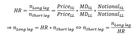
In order to implement this trade correctly, one must therefore ensure that the positive duration contribution from the purchase of the short-term bond futures is offset as exactly as possible by the sale of the long-term ones, such that a net duration neutrality is achieved. The number of futures contracts to be bought (long leg) and sold (short leg) can be determined using the following two formulas.
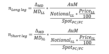
n long leg: Number of contracts of the future to be bought for the long leg (LL)
n short leg: Number of contracts of the future to be sold for the short leg (SL)
AuM: Asset under management of the portfolio denoted in the portfolio’s currency
MD: Desired absolute change of the portfolio’s modified duration (MD) denoted as a percentage
MD LL: Ask modified duration of the LL future denoted as a percentage
MD SL: Bid modified duration of the SL future denoted as a percentage
Price LL: Ask price of the LL future
Price SL: Bid price of the SL future
Notional LL: Notional amount of the LL future
Notional SL: Notional amount of the SL future
Spot PC/FC: Spot exchange rate between the portfolio’s currency (PC) and the futures’ currency (FC) denoted in units of the FC per one unit of the PC
The ratio of n long leg to n short leg is defined as the hedge ratio (HR). It denotes how many contracts of the LL future have to be bought given that one assumes some real number for n short leg or vice versa. Therefore, the following holds true:
The most practical way to bet on a steepening of the yield curve would be to invest in a fund that implements the strategy described above by the means of futures contracts. Care should be taken to select the right combination of tenors. Theoretically, it would also be possible to buy and sell the respective sovereign bonds directly. The problem with this method is that it is difficult to borrow bonds in order to be able to sell them. This restriction is so severe that this method would either not be available or simply too expensive.
Conclusion
The term structure of interest rates is determined by the yield of the bonds depending on the time to maturity, whereby the yield is composed of the “risk-free” interest rate and the risk premia. The level, slope and curvature determine the shape of the yield curve, which can be normal, flat or inverse. There are several theories which try to explain these shapes. Currently, the yield curves of some countries are so flat or inverse that they offer a great opportunity to bet on a steepening of them.
For a glossary of technical terms, please visit this link: Fund Glossary | Erste Asset Management
Legal note:
Prognoses are no reliable indicator for future performance.
[1] Litterman, R., Scheinkman, J. (1991). Common factors affecting bond returns. The Journal of Fixed Income 1 (1), 54-61.
[2] Modena, M. (2008). A macroeconomic analysis of the latent factors of the yield curve: Curvature and real activity. Financial Econometrics Modeling: Derivatives Pricing, Hedge Funds and Term Structure Models, 121-146.
[3] Moench, E. (2010). Term structure surprises: the predictive content of curvature, level, and slope. Journal of Applied Econometrics, 27 (4), 574–602.
Legal disclaimer
This document is an advertisement. Unless indicated otherwise, source: Erste Asset Management GmbH. The language of communication of the sales offices is German and the languages of communication of the Management Company also include English.
The prospectus for UCITS funds (including any amendments) is prepared and published in accordance with the provisions of the InvFG 2011 as amended. Information for Investors pursuant to § 21 AIFMG is prepared for the alternative investment funds (AIF) administered by Erste Asset Management GmbH pursuant to the provisions of the AIFMG in conjunction with the InvFG 2011.
The currently valid versions of the prospectus, the Information for Investors pursuant to § 21 AIFMG, and the key information document can be found on the website www.erste-am.com under “Mandatory publications” and can be obtained free of charge by interested investors at the offices of the Management Company and at the offices of the depositary bank. The exact date of the most recent publication of the prospectus, the languages in which the fund prospectus or the Information for Investors pursuant to Art 21 AIFMG and the key information document are available, and any other locations where the documents can be obtained are indicated on the website www.erste-am.com. A summary of the investor rights is available in German and English on the website www.erste-am.com/investor-rights and can also be obtained from the Management Company.
The Management Company can decide to suspend the provisions it has taken for the sale of unit certificates in other countries in accordance with the regulatory requirements.
Note: You are about to purchase a product that may be difficult to understand. We recommend that you read the indicated fund documents before making an investment decision. In addition to the locations listed above, you can obtain these documents free of charge at the offices of the referring Sparkassen bank and the offices of Erste Bank der oesterreichischen Sparkassen AG. You can also access these documents electronically at www.erste-am.com.
Our analyses and conclusions are general in nature and do not take into account the individual characteristics of our investors in terms of earnings, taxation, experience and knowledge, investment objective, financial position, capacity for loss, and risk tolerance. Past performance is not a reliable indicator of the future performance of a fund.
Please note: Investments in securities entail risks in addition to the opportunities presented here. The value of units and their earnings can rise and fall. Changes in exchange rates can also have a positive or negative effect on the value of an investment. For this reason, you may receive less than your originally invested amount when you redeem your units. Persons who are interested in purchasing units in investment funds are advised to read the current fund prospectus(es) and the Information for Investors pursuant to § 21 AIFMG, especially the risk notices they contain, before making an investment decision. If the fund currency is different than the investor’s home currency, changes in the relevant exchange rate can positively or negatively influence the value of the investment and the amount of the costs associated with the fund in the home currency.
We are not permitted to directly or indirectly offer, sell, transfer, or deliver this financial product to natural or legal persons whose place of residence or domicile is located in a country where this is legally prohibited. In this case, we may not provide any product information, either.
Please consult the corresponding information in the fund prospectus and the Information for Investors pursuant to § 21 AIFMG for restrictions on the sale of the fund to American or Russian citizens.
It is expressly noted that this communication does not provide any investment recommendations, but only expresses our current market assessment. Thus, this communication is not a substitute for investment advice.
This document does not represent a sales activity of the Management Company and therefore may not be construed as an offer for the purchase or sale of financial or investment instruments.
Erste Asset Management GmbH is affiliated with the Erste Bank and austrian Sparkassen banks.
Please also read the “Information about us and our securities services” published by your bank.